In the second blog post of this series related to the Blast Furnace Diagram, we explore some variations of the diagram constructed in the first blog post, while sticking to carbon as the only reducing agent in the system. This blog post was written in collaboration with Klaus Hack.
The first diagram that we will generate is similar to the one of the first blog article, but now we include graphite as a possible phase for carbon. We still consider only stoichiometric condensed substances in the calculation, but we are going to include some additional phases, that were not included before. The set-up on the “Components” window is basically the same as it was before. In the case of the “Menu” window, in the present case, we include all possible gas species. As for the liquid compound species, we adopt the following selection, like depicted on Figure 1.
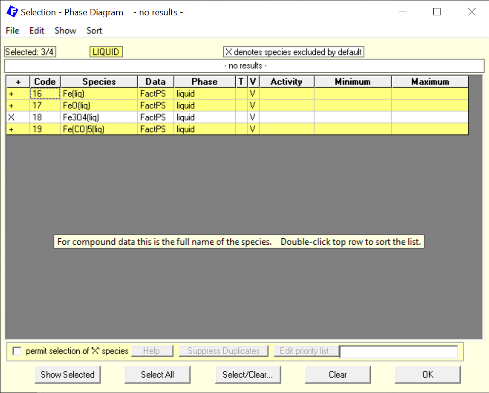
Figure 1 – Selection of the pure stoichiometric liquids
Notice that now, we have selected FeO(l) and also Fe(l) as possible species. For the solid compound species, we select them according to what is shown on Figure 2.
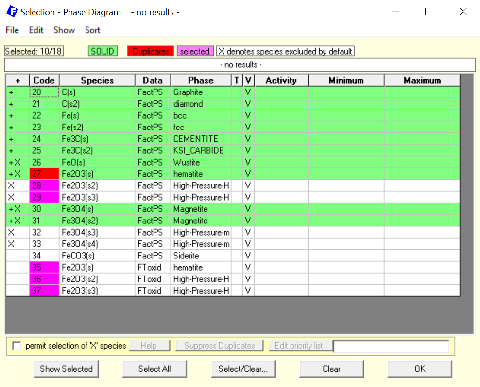
Figure 2 – Selection of the pure stoichiometric solids
Notice that now, we have included the different phases of pure solid carbon and also the different phases of pure solid iron. In the addition, stoichiometric FeO (Wustite), Fe3O4 (Magnetite) and Fe2O4 (Hematite) are also selected.
On the “Variables” window, we also change the set-up a little, to be able to look at a larger range of temperatures, see Figure 3.
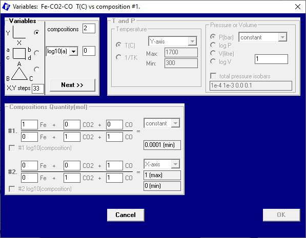
Figure 3 – Setting the axes variables and their ranges as well as constant variables
The following diagram is calculated after clicking the “Calculate” button. (Figure 4).
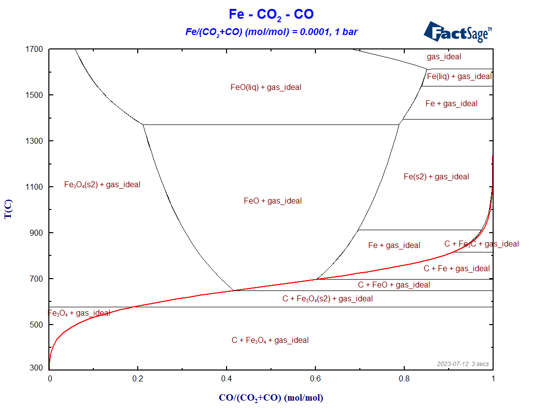
Figure 4 – The BF-diagram for the settings described above (red =Boudouard curve)
The main difference between this diagram and the corresponding one of the first blog post is, of course, the presence of carbon as graphite in it. The Boudouard-curve (in red) separates the regions in which graphite is a stable phase (below the curve) from those regions where graphite is thermodynamically not stable. In addition to this, different phases, that were not present in the first blog post, show up for Fe, FeO and Fe3O4. This leads to a division of the phase diagram into a number of new phase regions.
The classical Baur-Glässner diagram that was shown in the first blog article only takes stoichiometric condensed phases into account. Now let us take a look at what happens when we treat the system properly, i.e. including solution phases. It must be noted that except for graphite all phases are solution phases: Liquid Fe as well as BCC and FCC Fe, and also all the oxide phases. However, we will do so in two steps: First we will include only the oxide solution phases. In order to be able to do this, we must include the FToxid database in the “Data Search” window, as depicted in Figure 5.
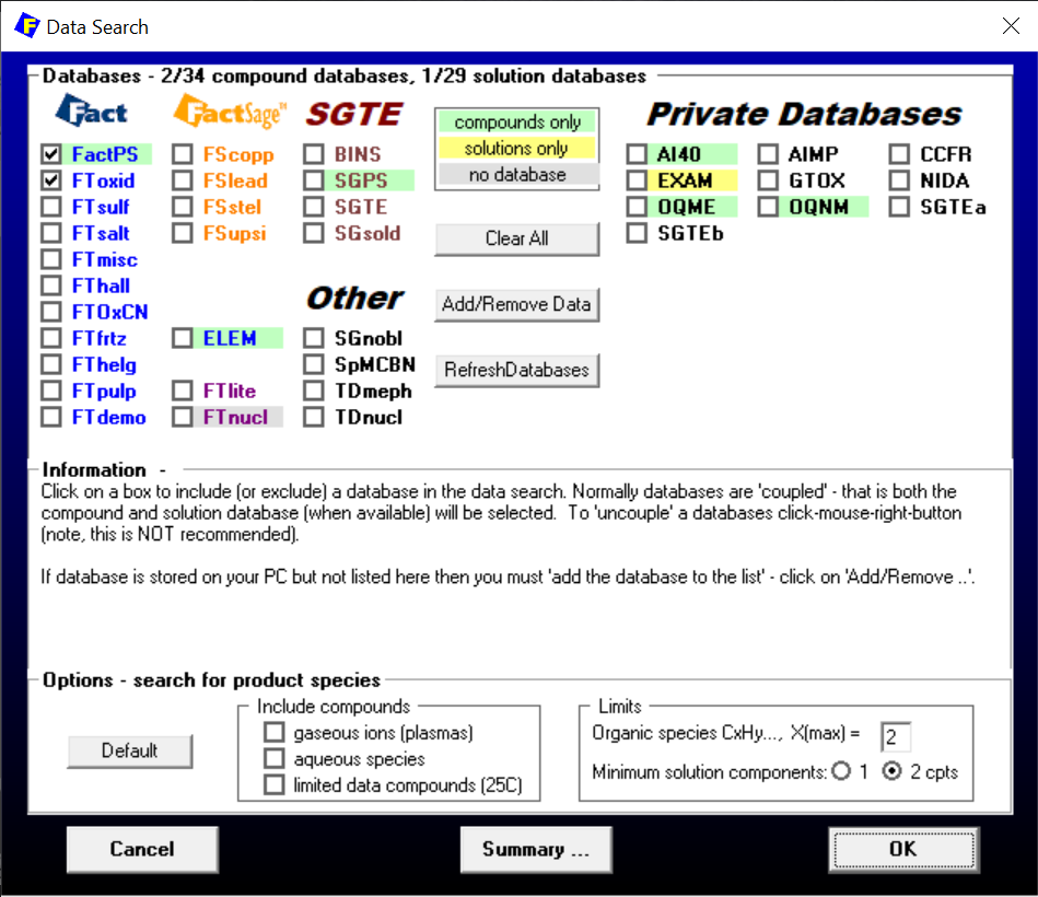
Figure 5 – The Data Search window is used to include both the Fact PS and the FTOxid database in the calculations
Then we select phases on the Menu Window like on Figure 6.
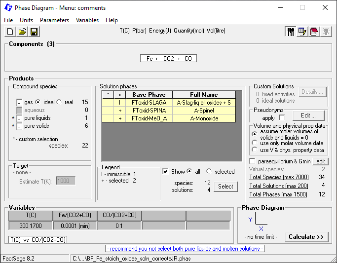
Figure 6 – Selection of the phases to be used in the calculation
Notice that we include all possible gas species and also all possible oxide solution phases. As for the pure liquids, we include only Fe(l). In the case of the pure solids, we include only non-oxide compounds species (i.e. Fe BCC and FCC as well as C graphite and Fe3C), since the oxide phases are solution phases. By clicking on “Calculate”, we generate the following diagram:
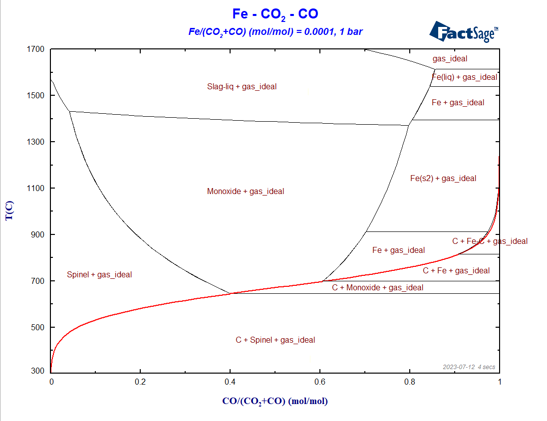
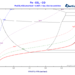
Figure 7 – The BF-diagram incorporating all oxide phases as solutions
Notice the change in shape and size of the phase regions caused when considering the oxide solution phases in the calculation. This results from the fact that both Monoxide and Slag exhibit considerable deviations from the stoichiometric FeO composition.
Next, we show how to include isoactivity lines for the phase activity of C(graphite) on the diagram. For this, we need to come back to the Menu Window (Figure 6 above). Once we are there, we right click on the word “pure solids” at the left side of the window with the mouse. The list of solid species should appear, we right click then at the first column of the line corresponding to C(graphite) and then on “Z-isoactivities” of the menu that shows up (Figure 8).
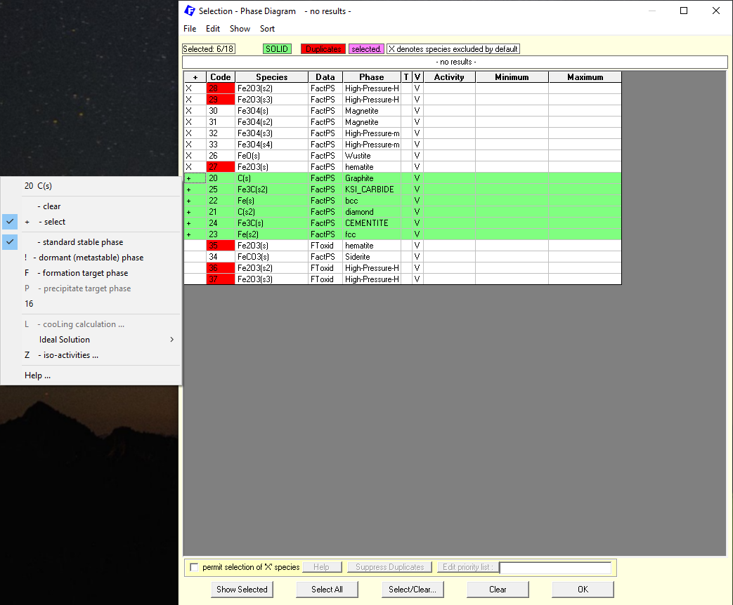
Figure 8 – Setting the activity values of the desired iso-activity lines
On the entry field that shows up, we enter the values for a(C(graphite)): 0.1, 1e-2, 1e-4 and 1e-6. If we now click on “OK” and recalculate from the Menu Window, the last phase diagram will show up now with the isoactivity lines.
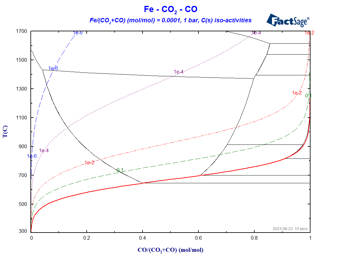
Figure 9 – The BF-diagram as in Fig. 7, but now also including iso-activity lines for C
Note that these lines all lie in the range above the Boudouard line. On and below the line the activity of C(graphite) is equal to 1. The Boudouard-line is the ZPF (zero-phase-fraction) line for the C(graphite) phase. The area below it is the area of stability of this phase, i.e. the activity is everywhere equal to one, no matter which other phase(s) are stable too.
That is it for the time being. In the next blog post, we will show the influence of the total pressure and also the effect of making all metallic phases solution phases on this kind of diagrams. See you again in the next part of this series of blog posts!
This post is part of our series Constructing a Blast Furnace Diagram with FactSage: