FactSage databases constitute the largest set of evaluated and optimized thermodynamic databases for inorganic systems in the world [1]. However, in case your system of interest is not (fully) covered by commercial databases, the development of own, i.e. private, databases might be required. This blogpost outlines how you can create a private database in FactSage as input for the Calphad Optimizer. While the procedure applies to any binary and higher order systems, the binary metallic Pb-Sn system is used as example.
The Calphad Optimizer, our new module to facilitate the development of thermodynamic databases using the Calphad methodology, helps you to derive a set of self-consistent thermochemical parameters for optimal reproduction of known experimental data (click here for more information: https://gtt-technologies.de/2022/09/calphad-optimizer/).
To following database requirements have to be met in the current version of the Calphad Optimizer (v.1.3.0):
- The database is unencrypted (private)
- The database contains all relevant stoichiometric phases
- All functions to describe solution end members are available
- The database contains all relevant solution phases and these are described utilizing suitable thermochemical models
- Interaction parameter for optimization are created
In the following, the sequence above is followed to demonstrate how to create the first private database paving the way for the optimization process in Calphad Optimizer.
Step 1: Creating a private compound database
Open the compound module in FactSage and navigate to “File => New Database…”. Select the respective folder, in which you want to save your new database and provide a meaningful name. The first four letters of the name are taken as the unique nickname in FactSage. For the Pb-Sn system, you could simply name the database PBSN. You have now created your first private unencrypted compound database as indicated by the “r/w” symbol in the compound module. Great!
(see also slides 1-4 in the help section of the compound module)
Step 2: Adding all relevant stoichiometric phases
However, so far your database is still empty. What stoichiometric phases do you need? First you should add the system components of the database, preferably in their reference states, so fcc Pb and bct Sn in our example case. But where do we get the data? This can be a blogpost on its own and is not the major focus here, so just a few words: for most typical pure substances, high quality data is already collected in the pure substance databases FactPS and SGPS. In case you are interested in less well-investigated pure substances, our aiMP & aiOQ databases might be of interest for you (https://gtt-technologies.de/wp-content/uploads/2022/08/AIMP_AIOQ_v5_Docu.pdf). By entering the formula of interest (“Pb”) in the Compound module, all databases containing a phase with that stoichiometric formula are indicated by the [+] sign appearing next to the database name. As there are likely multiple databases to select from, the process of selecting the correct source should be guided by e.g. known application areas of the databases. After selecting the source of the pure substance data, you can transfer the data from the otherwise encrypted database to your private one using drag & drop in the Compound module, as exemplarily shown below for the data for Pb from SGPS. Note that you automatically copy all phases for the selected compound. Hence, for Pb from SGPS, Pb(S1=fcc), Pb(L1=liq) and Pb(G1=gas) are all copied into your database.
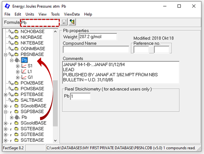
Figure 1: Copy pure substance data to your private database in the Compound module.
Depending on the system of interest, more pure substance data, e.g. for stoichiometric intermetallic phases, is needed but in case of Pb-Sn, no stoichiometric phases exist. Hence, step 2 is done and your private database contains all relevant stoichiometric phases after copying the data for Pb and Sn.
(for transferring data, see also slides 27 ff. in the help section of the compound module)
(for adding new compound data, see also slides 5 ff. in the help section of the compound module)
Step 3: Creating the solution database
Now it is time to open also the solution module and to create a solution database for the Pb-Sn system. We suggest to provide the same name, PBSN, to ensure coupling of both databases upon loading.
(see also slide 3 in the help section of the solution module)
Step 4: Add all relevant functions to describe solution endmember
The next decisive question is which solution phases need to be modelled for the system of interest. In case of Pb-Sn, we have three relevant solution phases: bct, fcc & liquid, as depicted here: https://www.crct.polymtl.ca/fact/phase_diagram.php?file=Pb-Sn.jpg&dir=SGTE2020.
For each solution phase, you need to describe the solution endmembers. Thus, a thermodynamic description of Pb and Sn in bct and fcc structure as well as in their liquid form is required, making it necessary to add these six functions (Pb(bct), Pb(fcc), Pb(liq), Sn(bct), Sn(fcc), Sn(liq)) to the solution database. When the data is available in the compound module, it is easy to copy it via drag and drop form the compound module to the functions section of the database in the solution module, as exemplarily shown here.
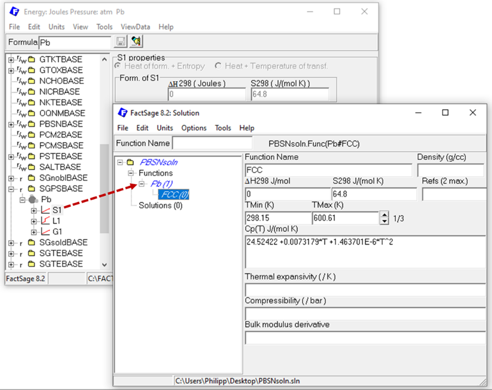
Figure 2: Copy compound data as functions from the Compound module to the Solution module to describe solution endmember.
Of course it is more difficult to find reliable and accurate data of solution endmembers in an un- or metastable form at standard conditions, e.g. Pb(bct) or Sn(fcc). However, pure element data for all stable and many metastable modifications can be found here [2] and already in FactSage format as SGUN in the FACTDATA folder of your FactSage installation. The drag&drop functionality in FactSage ensures that you can avoid errors frequently occurring in Calphad databases in TDB format. Besides, it is also possible to create new functions in the solution module based on data found, for example, in the literature. Our databases aiMP and aiOQ (https://gtt-technologies.de/wp-content/uploads/2022/08/AIMP_AIOQ_v5_Docu.pdf) also serve as an excellent starting point for stable or metastable endmembers not assessed experimentally.
After finding reliable data and adding all six missing functions to describe the solution endmembers for the Pb-Sn system, you can head to the next step.
(see also slides 12 ff. in the help section of the solution module – models and examples)
Step 5: Creating the solution phases
Move to the solution part of your database and perform a right-click to add a new solution. Provide a meaningful name, e.g. FCC in case of Pb-Sn, select the state and the model. Finding the right model to describe the phase is decisive and again, can be a at least a blogpost on its own and is not discussed in detail here. In FactSage a very extensive list of solution models is implemented and ready to be used by you. Insightful explanation and examples are provided in the help section of the solution module, so have a look there. For the simple Pb-Sn example, the one-lattice Redlich-Kister/Muggiano only model, short RKMP, could be a sensible selection for all three solution phases assuming that a second sublattice, e.g. to model interstitial defects, is not required.
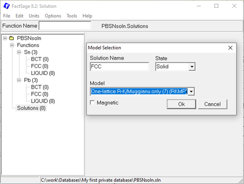
Figure 3: Creating new solution phases in the Solution module.
After creating all three solution phases, the sublattice species, Pb and Sn, need to be defined. Upon right-click on the just created sublattice species, the corresponding endmember of the respective solutions can be created. The next step is to assign the correct Gibbs energy function to the respective endmember, as exemplarily shown here in case of the Pb endmember for the FCC solution.
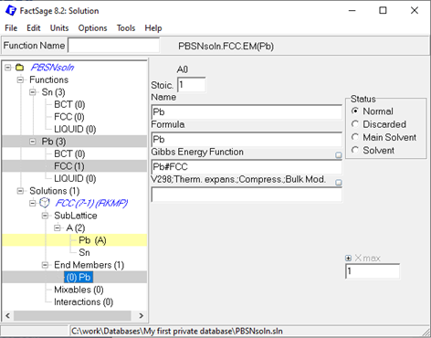
Figure 4: Assigning the Gibbs energy function to the solution endmembers in the Solution module.
Please note that it is also possible to combine multiple functions algebraically, which may help in case of endmembers that have complex stoichiometric composition and for which the Gibbs energy can be put together from multiple pure element functions, e.g. Fe3C->3*Fe#FCC + 1*C#Graphite.
In case of Pb-Sn, you can simply follow the same procedure for the Sn endmember of FCC and, of course, for the BCT and Liquid solution. Done? Great! You should now have a solution database containing three solutions with all endmembers described, as shown below:
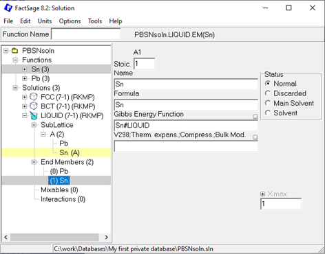
Figure 5: Pb-Sn solution database after setting up all three solution phases.
(see also slides 2 ff. for a description of the different models and slides 14 ff. for creating and
setting up solutions in the help section of the solution module – models and examples)
Hint for advanced users:
If it is anticipated that an adjustment of the Gibbs energy is needed when the system is assessed using Calphad Optimizer, it may be reasonable to add a function #a (unit enthalpy) and #bT (negative unit entropy). Thus, a typical Gibbs energy of formation expressed as ΔG = a + bT, e.g. ΔG = 1000 + 2T can be added to the Neumann-Kopp sum by adding 1000*#a +2*#bT.
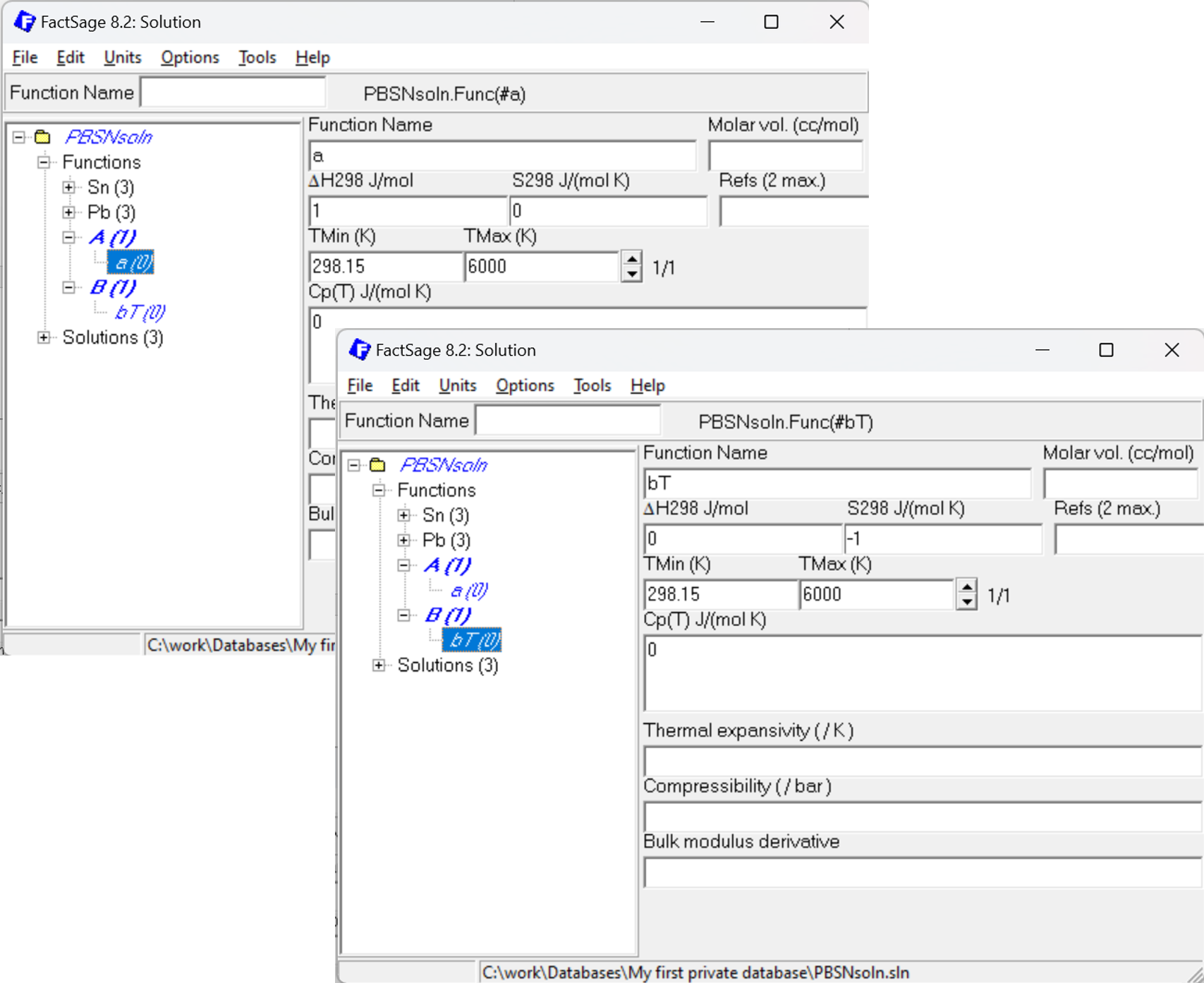
Figure 6: How to set up additional functions #a and #bT to describe Enthalpy and Entropy.
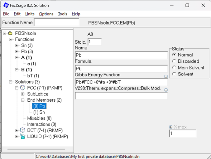
Figure 7: Gibbs Energy description of the fcc Pb Endmember using the additional #a and #bT functions.
Step 6: Creating interaction parameters
To describe the non-ideal interaction between the species within the just created solutions, the respective interaction parameters are required. Binary interactions are created in the solution module by marking the two sublattice species (holding the Ctrl key) and subsequent right-clicking on the marked species. For the Pb-Sn example, Bragg-Williams Redlich-Kister (RK) type interaction parameters, can easily be added that way:
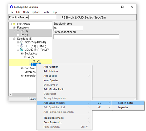
Figure 8: Adding a Bragg-Williams Redlich-Kister GE interaction parameter for the Pb-Sn liquid solution.
Since it is not possible to add interaction parameters at a later stage in the Calphad Optimizer (v.1.3.0), it might be helpful to directly add higher order (i=1,2…) RK interaction parameters to enable their inclusion in the subsequent optimization process. For the Pb-Sn example, two RK interactions (i=0 & 1), for all three solutions with a value of 0 can be added to the solution database. An example is shown here for the liquid solution (order i=1):
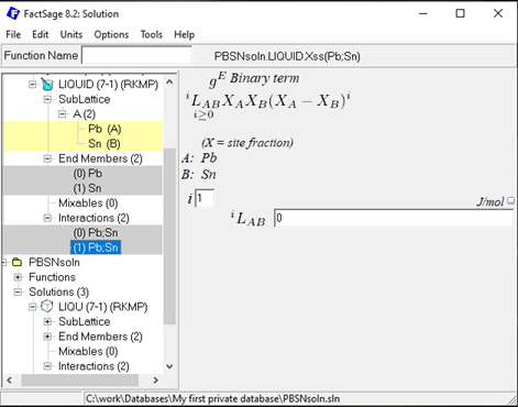
Figure 9: Second first order (i=1) Bragg-Williams Redlich-Kister GE interaction parameter for the Pb-Sn liquid solution.
After adding all interaction parameters, the private database for the Pb-Sn system now meets all requirements outlined above! Please note that the Calphad Optimizer (v.1.3.0) currently requires .dat as the input format requiring another simple file conversion, which can be performed in the Equilib module. A detailed explanation can be found in the Calphad Optimizer documentation (slide 18 ff.).
Have fun with the optimization. If you have any question concerning the Calphad Optimizer, please do not hesitate to contact us under calphad@factsage.com!
References
[1] Jung, I.-H., Van Ende, M.-A., 2020. Computational Thermodynamic Calculations: FactSage from CALPHAD Thermodynamic Database to Virtual Process Simulation. Metall. Mater. Trans. 50th Anniv. Collect. 51, 1851–1874.
[2] Alan Dinsdale, SGTE Data for Pure Elements, Calphad Vol 15(1991) pp. 317-425.