In this blog post we will see how to interpret the phase activity of a phase which does not form in equilibrium for a given temperature and pressure. For this, we will consider an Al-Cu alloy containing 0.01 mol% Cu at a temperature of 500°C and at a pressure of 1 atm and we will see how far we are from forming θ-Al2Cu in terms of its phase activity and Gibbs free energy. In a previous post we analyzed this situation just by considering the corresponding phase diagram.
We are again using the Equilibrium Module of FactSage Edu. The choice of the database and of working units is the same as in the previous blog post. After choosing the database and defining the units, we define the reactants on the reactants window as shown in Figure 1.
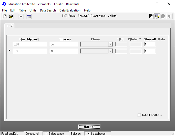
Figure 1
Then we click on “Next” and define the phases to be considered and the temperature and pressure for the calculation as depicted in Figure 2.
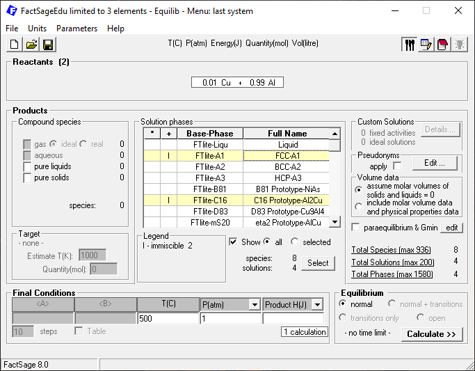
Figure 2
When we click on calculate, we get then the results shown on Figure 3.
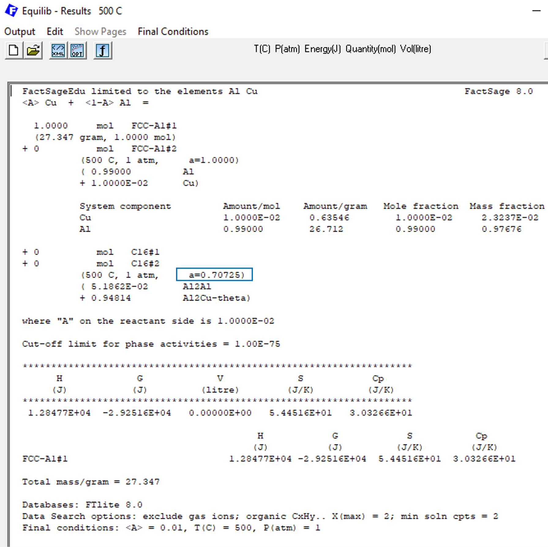
Figure 3
Please notice in Figure 3 that the phase C16, that corresponds to the θ-Al2Cu phase, is not forming. This is expected from the phase diagram calculated on the previous blog post of this series. In Figure 3 we marked the value of the corresponding phase activity for the phase C16 with a blue square, this value being a=0.70725. Considering that unstable phases should have activities smaller than one, this value is consistent with the phase diagram. But how is this value calculated by FactSage?
To show the relationship between phase activity and Gibbs Energy, we need to plot the molar Gibbs Energies of the FCC and of the θ-Al2Cu phases as functions of their compositions for the considered temperature and pressure. In order to do this, we use the <A>-parameter (see the previous post on this topic as a reference) and we construct Figure 4, from the menu item Output > Plot > Plot Results.
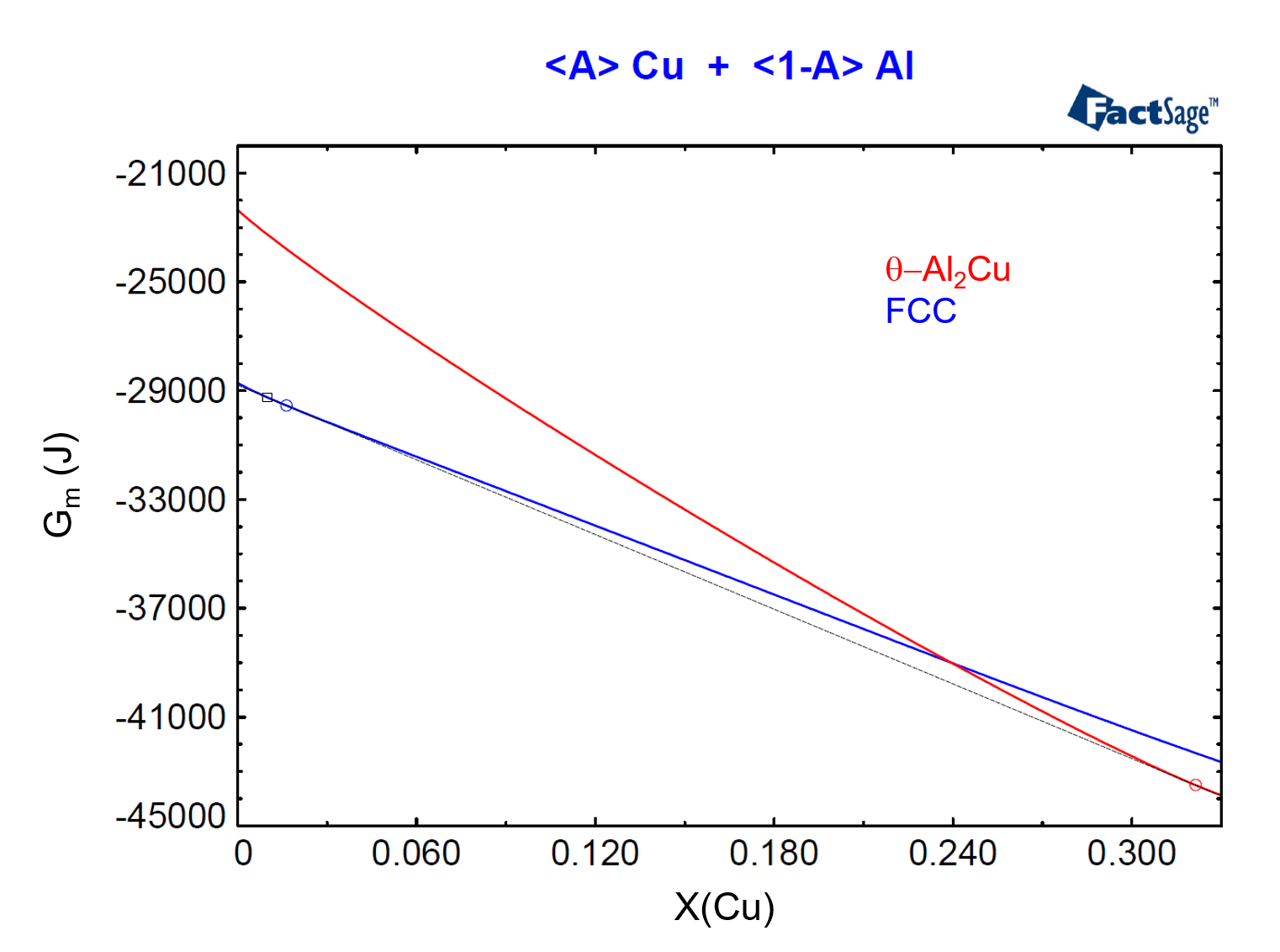
Figure 4
In Figure 4, we have drawn the common tangent line to the two Gibbs Energy curves. This common tangent defines the equilibrium compositions of the two phases, denoted by a blue circle and by a red circle, for the FCC and θ-Al2Cu phases respectively. Notice that the composition of the alloy, X(Cu) = 0.01, is located to the left of the blue circle, denoting that this alloy is in the region where only the FCC phase is stable.
Now we draw a line tangent to the Gibbs Energy curve for the FCC phase at X(Cu) = 0.01. The dashed blue line on Figure 5 shows this line. Then, two conditions are possible for an arbitrary phase which is thermodynamically represented by a new Gibbs energy curve. First, if the new curve touches the dashed blue line, an equilibrium between the corresponding phase and the FCC-phase with X(Cu) = 0.01 is possible. Second, if the new curve lies above this tangent for all compositions, then such phase is not stable against the FCC phase with X(Cu) = 0.01. The second condition corresponds to that of the θ-Al2Cu phase in the present situation. But how far is the θ-Al2Cu phase away from forming for this alloy composition, i.e. how much is the missing driving force for this phase to form?
To answer this question, we draw a tangent to the Gibbs Energy curve of the θ-Al2Cu phase which has the same slope of the tangent line of the previous paragraph. The dashed red line on Figure 5 shows this second line, which is tangent to the Gibbs Energy Curve of θ-Al2Cu at X=0.316. This defines the point on the Gibbs Energy curve of the θ-Al2Cu phase which is closest to the blue dashed line.
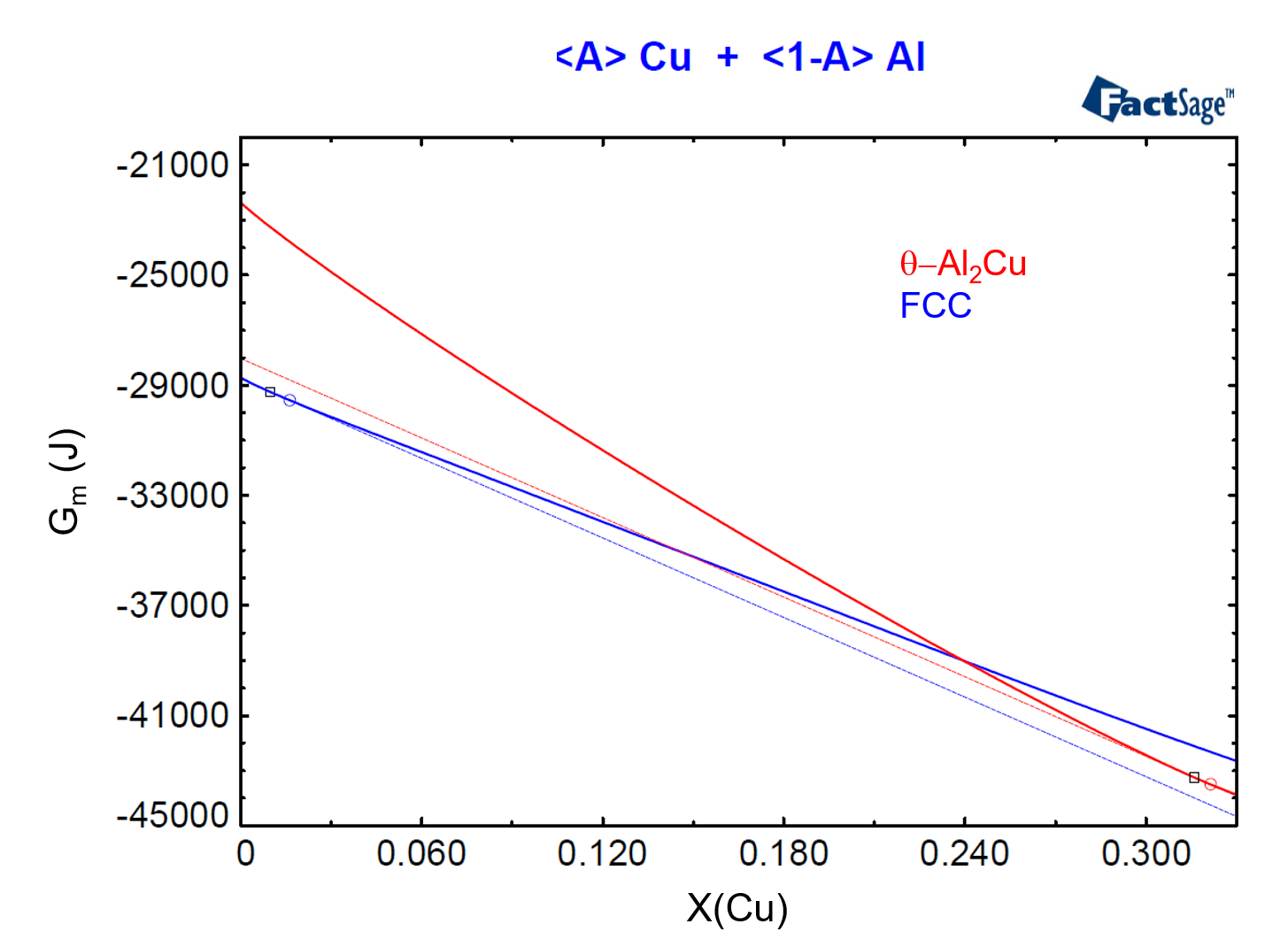
Figure 5
The vertical distance between the red and the blue dashed lines defines the value of the missing driving force we are searching for. On Figure 6 we zoom in on the region around X(Cu)=0.316 of the diagram of Figure 5. If we now use the numbers generated by FactSage to calculate the vertical difference between the Gibbs Energies given by the two lines at any X(Cu) value, as in the expression below
$${\Delta}G = G_{FCC} – G_{Al_2Cu}$$
we come to the value -742.18 J. This value is represented by the arrow on Figure 6, which corresponds to the vertical distance between the two tangent lines at X(Cu) = 0.316.
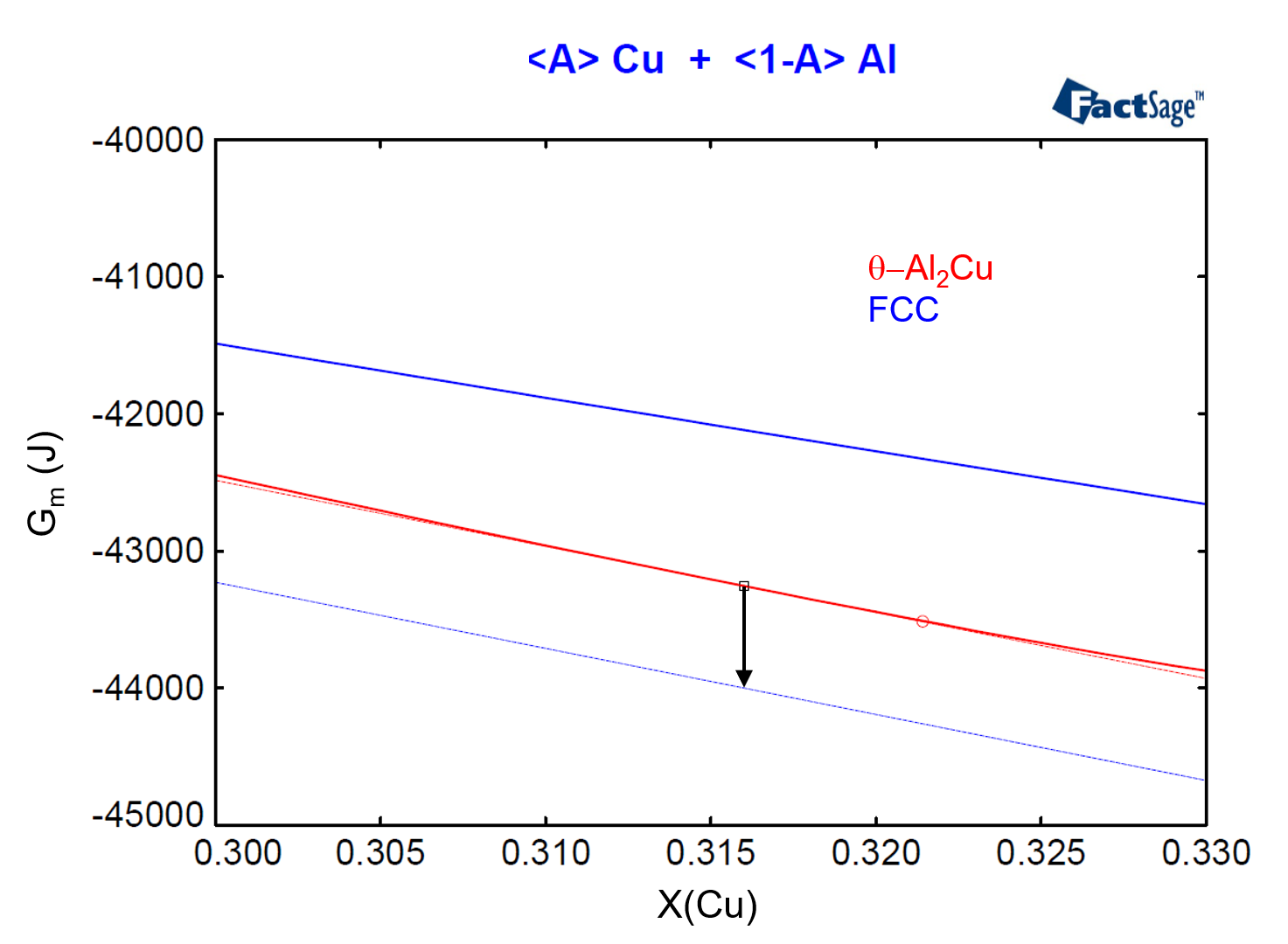
Figure 6
The calculation above results in a value for the “missing” Gibbs Energy per one mole of atoms in the θ-Al2Cu phase. If we now multiply this value by three, to obtain the Gibbs energy variation for one mole of formula unit of the θ-Al2Cu phase and insert then the new value into the expression below
$${\Delta}G^* = RT ln (a_{Al_2Cu}) = -2226.54 J$$
we obtain an equation, that can be solved for a(Al2Cu). The resulting value for a(Al2Cu) is equal to 0.70725, which is the value shown on the FactSage Result screen of Figure 3. This is how FactSage determines the phase activity of a non-equilibrium phase.