As of version 3.0.0, ChemApp is able to perform one-dimensional phase mapping calculations. Users of ChemSage will very likely be familiar with this feature already, since it is very useful in phase equilibrium calculations. One-dimensional phase mapping is generally used to search for phase boundaries within the range of a given variable (temperature, pressure, or composition). With only a few lines of code it allows the programmer to automatically locate every phase boundary within a specified range.
Using one-dimensional phase mapping thus makes it very easy to find phase boundaries in a variety of phase diagrams, such as those with temperature/composition (T/x), pressure/composition (P/x), and temperature/pressure (T/P) as axes.
The following program demonstrates one-dimensional phase mapping calculations in a T/x and a T/P diagram.
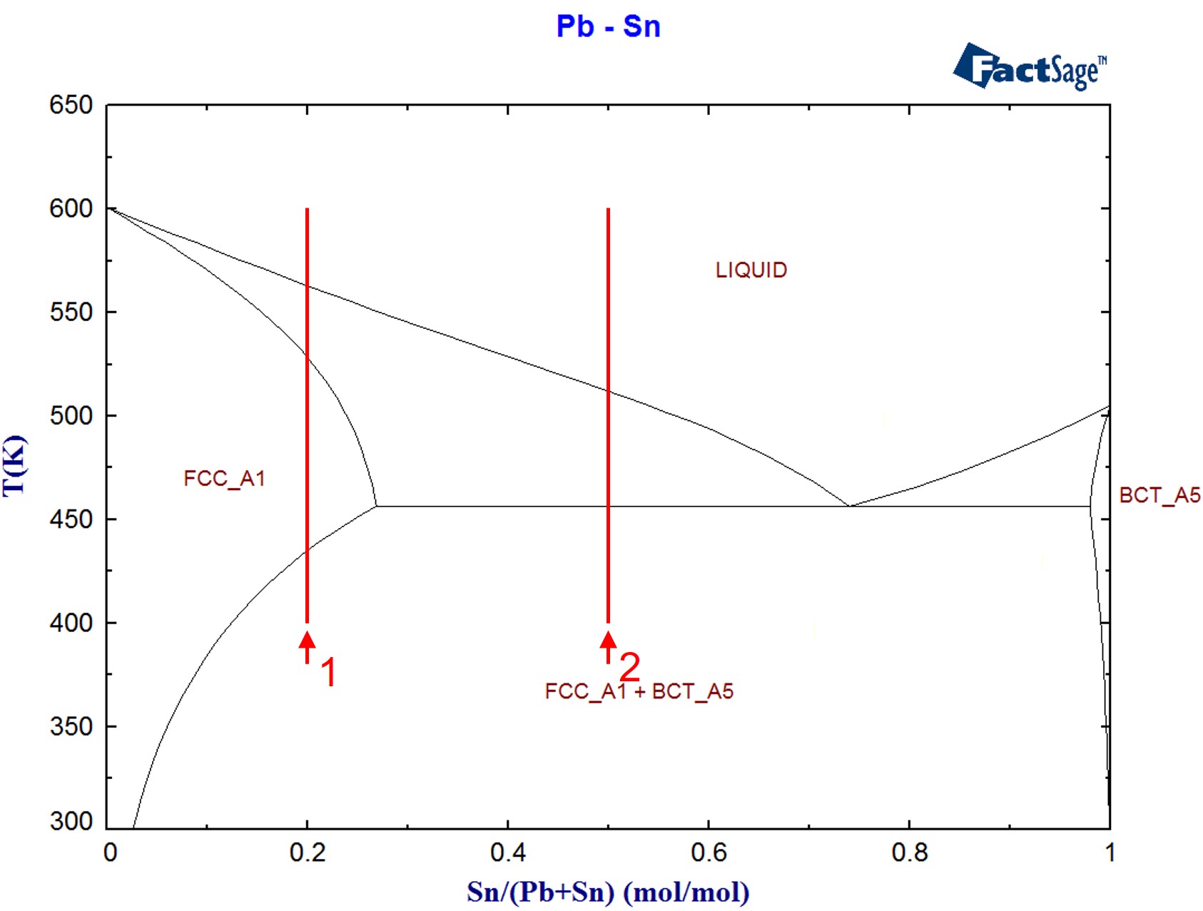
The system Pb-Sn, already described in the example Phase equilibria and phase target calculations, is used to demonstrate the calculation of two one-dimensional phase maps in a T/x diagram, with the temperature as the search variable. The lines marked 1 and 2 in Figure 1 indicate the range within which the phase boundaries will be searched.
Figure 1: The Pb-Sn phase diagram (calculated using FactSage)
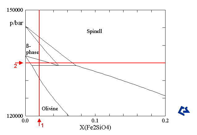
For the system System Fe2SiO4-Mg2SiO4, a T/P phase diagram has been calculated using ChemSage. A section of it is shown in Figure 2. In the course of the following example program, two one-dimensional phase maps will be calculated in this phase diagram, using first pressure (line 1) and then composition (line 2) as the search variable.
Figure 2: The Fe2SiO4-Mg2SiO4 pressure/composition phase diagram at 1000 (calculated using ChemSage)
In this example emphasis is placed on demonstrating the method of finding the phase boundaries within the ranges of the search variables specified. For all the phase boundaries found, only minimal tabular information is output. For the first phase map it is also demonstrated which results need to be collected to produce a graphical representation of the phase map.
The following one-dimensional phase maps will be calculated:
- In the T/x phase diagram Pb-Sn, two maps with temperature as the search variable (lines 1 and 2 in Figure 1). The first one of these two will be shown graphically.
- In the T/P phase diagram Fe2SiO4-Mg2SiO4, a map with pressure as the search variable (line 1 in Figure 2)
- For the same system and phase diagram, a map with the concentration as search variable (line 2 in Figure 2)
C One-dimensional phase mapping calculations

C Note that this program contains target calculations,
C which cannot be performed with the 'light' version of ChemApp

C Subroutine BSORT implements a simple bubble sort algorithm. It is
C used to sort the array of temperature values for which phase
C equilibria are to be calculated.
      SUBROUTINE BSORT(NPTS, TARRAY, NUSED)
      IMPLICIT NONE
      INTEGER NPTS, NUSED
      DOUBLE PRECISION TARRAY(NPTS)
      INTEGER I,J
      DOUBLE PRECISION TEMP

C Sort the first NUSED elements of TARRAY, which has a total number
C of NPTS elements, in ascending order
      DO I=1,NUSED
         DO J=I+1, NUSED
            IF(TARRAY(I).GT.TARRAY(J)) THEN
               TEMP=TARRAY(I)
               TARRAY(I)=TARRAY(J)
               TARRAY(J)=TEMP
            ENDIF
         ENDDO
      ENDDO
      RETURN
      END


C Subroutine PSP prints the value of the 'search variable' (temperature,
C pressure, or composition), the names of the stable phases, and their
C amounts. It is used after every call to TQMAP.
      SUBROUTINE PSP(VALUE1, VALUE2)
      IMPLICIT NONE
      DOUBLE PRECISION VALUE1, VALUE2, AMT, ACT
      CHARACTER PNAME*24, PSTAT*24
      INTEGER NPHASE, I, NOERR

C If the second parameter to PSP is zero, we only need to print the
C first one.
      IF (VALUE2 .NE. 0.D0) THEN
         WRITE(6,FMT='(2F12.3)') VALUE1, VALUE2
      ELSE
         WRITE(6,FMT='(F12.2)') VALUE1
      ENDIF

C Find out how many phases we have in the system
      CALL TQNOP(NPHASE, NOERR)

C For every phase, check whether its activity is unity
      DO I=1, NPHASE
         CALL TQGETR('AC ', I, 0, ACT, NOERR)
         IF (ACT .GE. 1.D0) THEN

C Check if the phase has the status ENTERED, otherwise (i.e. when the
C status of the phase is DORMANT) it might have an activity > 1 and
C still have an equilibrium amount of zero:
            CALL TQGSP(I, PSTAT, NOERR)
            IF (PSTAT .EQ. 'ENTERED') THEN

C If it is stable _and_ its status is ENTERED, get the name of that
C phase...
               CALL TQGNP(I, PNAME, NOERR)

C ...and its equilibrium amount...
               CALL TQGETR('A ', I, 0, AMT, NOERR)

C ... and print both:
               WRITE(*,FMT='(27X,A,F8.2)') PNAME, AMT
            ENDIF
         ENDIF
      ENDDO
      RETURN
      END


      PROGRAM CAF104

      IMPLICIT NONE

      INTEGER NOERR, NUMCON, BCT2, IPB, ISN, IPFESI, IPMGSI, ISLITE,
     *     ICONT, RESNO, NUSED, ASIZE, ITEMP

      PARAMETER(ASIZE = 100)

      DOUBLE PRECISION VALUE1, VALUE2, VALS(2), TARRAY(ASIZE),
     *     EPS, AMTS(4), ACTS(4)

      PARAMETER(EPS = 1.E-3)

      NUSED = 0

C Initialise ChemApp
      CALL TQINI(NOERR)

C Open the thermochemical data-file pbsn.dat (system Pb-Sn)
C for reading
      OPEN(10, FILE='pbsn.dat', STATUS='OLD', IOSTAT=NOERR)
      IF (NOERR .NE. 0) THEN
         WRITE(*,*) 'ERROR: Cannot open data-file.'
         STOP
      ENDIF

C Read data-file
      CALL TQRFIL(NOERR)

C Close data-file
      CLOSE(10)

C Check if we are working with the 'light' version.
C If we do, omit the following target calculation(s).
      CALL TQLITE(ISLITE, NOERR)
      IF (ISLITE .EQ. 1) THEN
         WRITE(*,FMT='(3(1X,A,/))')
     *     '*** Target calculations have been omitted here,',
     *     '*** since they are not possible with the ',
     *     '*** ''light'' version of ChemApp.'

      ELSE

C The data-file for system Pb-Sn contains a second copy of the BCT_A5
C phase, because of the inherent metastable miscibility gap. Since this
C miscibility gap will stay metastable under the conditions used in this
C example, we will eliminate the second copy of that phase, which means
C it will be disregarded completely in the following calculations.
      CALL TQINP('BCT_A5#2', BCT2, NOERR)
      CALL TQCSP(BCT2, 'ELIMINATED ', NOERR)

C Determine the index numbers for the system components Pb and Sn
      CALL TQINSC('Pb ', IPB, NOERR)
      CALL TQINSC('Sn ', ISN, NOERR)

C As indicated in Figure 1, label "1", the first phase map
C should be done with the temperature as the search variable, for
C X(Sn)=0.2.

C Set the incoming amounts for the Sn and Pb
      CALL TQSETC('IA ', 0, ISN, 0.2D0, NUMCON, NOERR)
      CALL TQSETC('IA ', 0, IPB, 0.8D0, NUMCON, NOERR)

C VALS is passed to TQMAP; this array of 2 DOUBLE PRECISION variables
C contains the lower and upper values of the search variable. Note that
C the first two calls to TQMAP _always_ calculate the equilibria at
C VALS(1) and VALS(2), and thus do _not_ constitute phase boundaries.
      VALS(1) = 400.D0
      VALS(2) = 600.D0

C The purpose of the array TARRAY is to hold the temperature values at
C which the equilibria will be calculated later. This set of temperature
C values consists of
C 1) a number of evenly spaced temperature intervals,
C 2) and the temperatures at which TQMAP finds phase boundaries.

C Part of the array is first filled with evenly spaced temperature
C intervals. As upper and lower values we use the same values as we did
C for the initialisation of VALS(1) and VALS(2) above. The variable
C NUSED keeps track of how many items of the array are actually used:
      DO ITEMP = 400, 600, 10
         NUSED = NUSED + 1
         TARRAY(NUSED) = ITEMP
      ENDDO

C RESNO keeps track of the number of results we get from TQMAP. This
C allows us to ignore the first two temperatures TQMAP reports. As
C indicated above, the first two calls to TQMAP do _not_ give us
C information about a phase boundary, but on the state at the lower and
C upper end of the search interval (i.e. at VALS(1) and VALS(2)). Since
C we have these temperatures in our temperature array TARRAY already
C (see the DO loop above), we only need to pay attention when we
C retrieve the third and any subsequent result with TQMAP.
      RESNO = 0

C First call to TQMAP. Note the option 'TF ', where 'T' indicates that
C temperature is the search variable, and 'F' ('first') that it is the
C first call to TQMAP for the current phase map. The variable returned
C through ICONT with every call to TQMAP will allow us to decide whether
C more calls to TQMAP are necessary. Since this is only the first call
C to TQMAP, we know anyway that we have to continue.
      CALL TQMAP('TF ',0,0,VALS,ICONT,NOERR)
      RESNO = RESNO + 1

C Get the temperature. Since it is the first call to TQMAP, we _know_
C that this will be the value of VALS(1)
      CALL TQGETR('T ',0,0,VALUE1,NOERR)

 100  FORMAT(1X,A,T28,A,T50,A)

C Print a header for the table to come.
      WRITE(*,FMT=100) 'Temperature/K', 'Stable phases', 'Amount/mol'

C Call PSP (print stable phases), passing the value for the temperature
C we just retrieved. PSP will print a formatted entry for the result
C table.
      CALL PSP(VALUE1, 0.D0)

C TQMAP is called again. Note the option 'TN ', where 'T' indicates that
C temperature is the search variable, and 'N' ('next') that it is _not_
C the first call to TQMAP for the current phase map.
 20   CALL TQMAP('TN ',0,0,VALS,ICONT,NOERR)
      RESNO = RESNO + 1

C Get the temperature.
      CALL TQGETR('T ',0,0,VALUE1,NOERR)

C If this is the second call to TQMAP, we know that the temperature
C retrieved here is VALS(2), and also that TARRAY already contains
C it. If, on the other hand, we are already retrieving our third or any
C subsequent result (checked through RESNO), we know it is a phase
C boundary.
      IF (RESNO .GT. 2) THEN

C What follows here is necessary because we would like to see the
C results of this one-dimensional phase map in a graph later.

C If we were just interested in the _position_ of this phase boundary,
C and thus the _value_ of the search variable (the temperature in this
C case), it would be enough to record this piece of information.
C However, since we would like to see a graphical representation of the
C phase map, we might not get the desired results if we just add the
C temperature found to TARRAY. Instead of calculating the equilibrium at
C the temperature just retrieved, we better calculate it at _two_
C temperatures: One slightly below, and one slightly above the
C temperature found. Thus these two temperatures are added to TARRAY
C instead of the exact temperature for the phase boundary (EPS has been
C defined using a PARAMETER statement at the beginning of the program):
         NUSED = NUSED + 1
         TARRAY(NUSED) = VALUE1 - EPS
         NUSED = NUSED + 1
         TARRAY(NUSED) = VALUE1 + EPS
      ENDIF

C Print the entry for the result table. For this purpose, we need the
C _exact_ temperature at the phase boundary, as determined by TQMAP:
      CALL PSP(VALUE1, 0.D0)

C The variable ICONT returned by TQMAP indicates whether we need to make
C any more calls to TQMAP, i.e. whether there are any more phase
C boundaries within the search interval we specified. If ICONT is
C positive, we need to continue.
      IF (ICONT .GT. 0) GOTO 20
Output:
 Temperature/K             Stable phases         Amount/mol
      400.00
                           BCT_A5#1                    0.06
                           FCC_A1                      0.94
      600.00
                           LIQUID                      1.00
      426.36
                           BCT_A5#1                    0.00
                           FCC_A1                      1.00
      505.37
                           LIQUID                      0.00
                           FCC_A1                      1.00
      560.01
                           LIQUID                      1.00
                           FCC_A1                      0.00
|
C When we arrive at this point of the program ICONT is zero, which tells
C us that there are no more phase boundaries left within the search
C interval we specified.

C The array TARRAY now contains all the temperatures at which we want to
C calculate the equilibria for our graphical phase map: the evenly
C spaced temperatures plus the two temperatures for every phase
C boundary: One slightly below and one slightly above the temperature of
C the original phase boundary.
C
C The only problem is that these temperatures are not in ascending
C order, since all the temperatures for the phase boundaries have simply
C been added to the end of the list of evenly spaced temperatures.
C
C Looking at the first and last 10 values of TARRAY reveals this:

 101  FORMAT('TARRAY(',I2,') = ',F12.5)
      DO ITEMP=1, NUSED
         IF ((ITEMP .LT. 10) .OR. (ITEMP .GT. (NUSED-10))) THEN
            WRITE(*,101) ITEMP, TARRAY(ITEMP)
         ENDIF
      ENDDO
Output:
TARRAY( 1) =    400.00000
TARRAY( 2) =    410.00000
TARRAY( 3) =    420.00000
TARRAY( 4) =    430.00000
TARRAY( 5) =    440.00000
TARRAY( 6) =    450.00000
TARRAY( 7) =    460.00000
TARRAY( 8) =    470.00000
TARRAY( 9) =    480.00000
TARRAY(18) =    570.00000
TARRAY(19) =    580.00000
TARRAY(20) =    590.00000
TARRAY(21) =    600.00000
TARRAY(22) =    426.35862
TARRAY(23) =    426.36062
TARRAY(24) =    505.36777
TARRAY(25) =    505.36977
TARRAY(26) =    560.00807
TARRAY(27) =    560.01007
|
C To have the values for the graph displayed properly later, we thus
C need to sort this array using the subroutine BSORT:
      CALL BSORT(ASIZE, TARRAY, NUSED)

C We are now ready to calculate the equilibria for all the temperatures
C in TARRAY. These equilibrium calculations now being performed are
C _not_ target calculations of any kind any more, that's why we reset
C _all_ previous conditions including all targets and target variables.
      CALL TQREMC(-2, NOERR)

C The following equilibria are to be calculated for the same alloy
C concentration of course, so we use the same incoming amounts again.
      CALL TQSETC('IA ', 0, ISN, 0.2D0, NUMCON, NOERR)
      CALL TQSETC('IA ', 0, IPB, 0.8D0, NUMCON, NOERR)
C The graphical representation of the one-dimensional phase map will be
C done using two x/y graphs: one displaying the phase amounts vs. the
C temperature, the other one the phase activities vs. the
C temperature. We will write two output data-files for this purpose:
C caf104_1.rst will contain the phase amounts, whereas caf104_2.rst will
C contain the phase activities.
      OPEN(11, FILE='caf104_1.rst', STATUS='unknown', IOSTAT=NOERR)
      IF (NOERR .NE. 0) THEN
         WRITE(*,*) 'ERROR: Cannot open result file.'
         STOP
      ENDIF

      OPEN(12, FILE='caf104_2.rst', STATUS='unknown', IOSTAT=NOERR)
      IF (NOERR .NE. 0) THEN
         WRITE(*,*) 'ERROR: Cannot open result file.'
         STOP
      ENDIF

C For every temperature in TARRAY, calculate the equilibrium:
      DO ITEMP=1, NUSED

         CALL TQSETC('T ', 0, 0, TARRAY(ITEMP), NUMCON, NOERR)

C Note again that these are regular equilibrium calculations, no targets
C are involved:
         CALL TQCE(' ', 0, 0, VALS, NOERR)

C Retrieve the equilibrium amounts of _all_ phases with a single call to
C TQGETR. Note that AMTS is an array of appropriate size
         CALL TQGETR('A ', -1, 0, AMTS, NOERR)

C Write the temperature plus the phase amounts to the first output
C data-file:
         WRITE(11,FMT='(5F15.10)') TARRAY(ITEMP), AMTS

C Retrieve the equilibrium activities of _all_ phases with a single call
C to TQGETR. Note that ACTS is also an array of appropriate size
         CALL TQGETR('AC ', -1, 0, ACTS, NOERR)

C Write the temperature plus the phase activities to the second output
C data-file:
         WRITE(12,FMT='(5F15.10)') TARRAY(ITEMP), ACTS
      ENDDO

C We have now calculated the equilibria for all temperature values in
C TARRAY and can close the two output data-files.
      CLOSE(11)
      CLOSE(12)
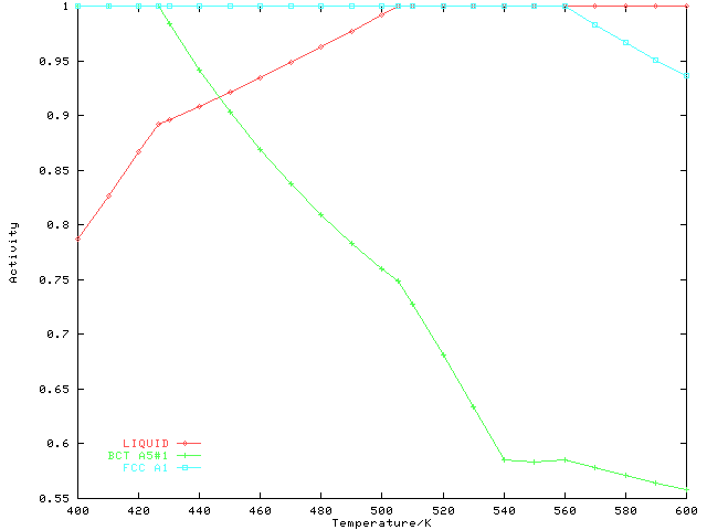
Figure 4: One-dimensional phase mapping calculation in the system Pb-Sn at xSn = 0.2: Calculated phase activities as a function of temperature. The kink in the activity curve for BCT_A5#1 near 540 K is due to the metastable miscibility gap in that phase.
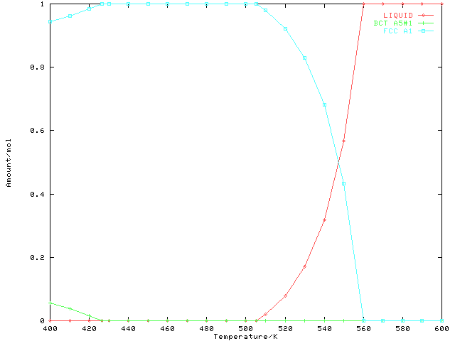
C When plotted, the two graphs, displaying the equilibrium phase amounts
C and phase activities vs. temperature look like Figures 3
C and 4.

C For the next one-dimensional phase mapping calculations we will only
C use tabular output. First, remove all previously set conditions.
      CALL TQREMC(-2, NOERR)

C We will now calculate another one-dimensional phase map in the same
C system, again with temperature as the search variable. The new
C alloy composition will cause TQMAP to find the eutectic.
      CALL TQSETC('IA ', 0, ISN, 0.5D0, NUMCON, NOERR)
      CALL TQSETC('IA ', 0, IPB, 0.5D0, NUMCON, NOERR)

C The temperature search interval used is the same:
      VALS(1) = 400.D0
      VALS(2) = 600.D0

C First call to TQMAP (note again the 'F' in the option parameter)
      CALL TQMAP('TF ',0,0,VALS,ICONT,NOERR)

C Retrieve the temperature, which we already know is VALS(1)
      CALL TQGETR('T ',0,0,VALUE1,NOERR)

C Print a header for the table to come.
      WRITE(*,FMT=100) 'Temperature/K', 'Stable phases', 'Amount/mol'

C Call PSP to print the information on the stable phases:
      CALL PSP(VALUE1, 0.D0)

C TQMAP is called with 'N' in the option parameter:
   30 CALL TQMAP('TN ',0,0,VALS,ICONT,NOERR)

C Get the temperature...
      CALL TQGETR('T ',0,0,VALUE1,NOERR)

C ... and print the entry for the result table:
      CALL PSP(VALUE1, 0.D0)
      IF (ICONT .GT. 0) GOTO 30
Output:
 Temperature/K             Stable phases         Amount/mol
      400.00
                           BCT_A5#1                    0.42
                           FCC_A1                      0.58
      600.00
                           LIQUID                      1.00
      454.56
                           BCT_A5#1                    0.33
                           FCC_A1                      0.67
      510.45
                           LIQUID                      1.00
                           FCC_A1                      0.00
|
C Note that the above table lists a 3-phase equilibria now, which for the
C current system means we found the eutectic temperature (compare this
C with the results for the same equilibrium determined in worked example
C 3: Phase equilibria and phase target calculations).

C So far we have calculated one-dimensional phase maps for a
C temperature/composition phase diagram, in our case keeping the
C composition (and implicitly the pressure) constant and using the
C temperature as the search variable. The next phase map we will
C calculate at a constant temperature, this time varying the
C pressure. For this purpose, we will use a different thermochemical
C data-file for the system Fe2SiO4-Mg2SiO4 which includes
C pressure-dependent Gibbs-energy data.

C Open the thermochemical data-file femgsio4.dat (system Fe2SiO4-Mg2SiO4)
C for reading
      OPEN(10, FILE='femgsio4.dat', STATUS='OLD', IOSTAT=NOERR)
      IF (NOERR .NE. 0) THEN
         WRITE(*,*) 'ERROR: Cannot open data-file.'
         STOP
      ENDIF

C Read data-file
      CALL TQRFIL(NOERR)

C Close data-file
      CLOSE(10)

C Determine the index numbers for the stoichiometric compounds Fe2SiO4
C and Mg2SiO4. These two phases will be used to define the incoming
C amounts for the next calculations. Note that they are included in the
C thermochemical data-file only for this purpose (to allow for a
C somewhat easier definition of incoming amounts), since the Gibbs
C energy functions for these two stoichiometric compounds are only
C dummies.
      CALL TQINP('Fe2SiO4 ', IPFESI, NOERR)
      CALL TQINP('Mg2SiO4 ', IPMGSI, NOERR)

C Select a composition of 2 mol-% Fe2SiO4, the rest is Mg2SiO4:
      CALL TQSETC('IA ', IPFESI, 0, 0.02D0, NUMCON, NOERR)
      CALL TQSETC('IA ', IPMGSI, 0, 0.98D0, NUMCON, NOERR)

C Select the range for the search variable, which is the pressure in the
C current case. We will search for any phase boundaries between 120 kbar
C and 150 kbar (see also the line marked '1' in Figure 2).
      vals(1) = 120000.D0
      vals(2) = 150000.D0

C The temperature is set to 1000 K
      CALL TQSETC('T ', 0, 0, 1000.D0, NUMCON, NOERR)

C First call to TQMAP. Note the option 'PF ', where 'P' indicates that
C pressure is the search variable, and 'F' that it is the first call
C to TQMAP for the current phase map.
      CALL TQMAP('PF ', 0, 0, VALS,ICONT, NOERR)

C Get the pressure. Since it is the first call to TQMAP, we _know_
C that this will be the value of VALS(1)
      CALL TQGETR('P ',0,0,VALUE1,NOERR)

C Print a header for the table to come.
      WRITE(*,FMT=100) 'Pressure/bar', 'Stable phases', 'Amount/mol'

C Call PSP (print stable phases), passing the value for the pressure
C we just retrieved. PSP will print a formatted entry for the result
C table.
      CALL PSP(VALUE1, 0.D0)

C TQMAP is called again. Note the option 'PN ', where 'P' indicates that
C temperature is the search variable, and 'N' that it is _not_ the first
C call to TQMAP for the current phase map.
   40 CALL TQMAP('PN ',0,0,VALS,ICONT,NOERR)

C Get the pressure.
      CALL TQGETR('P ',0,0,VALUE1,NOERR)

C Print the entry for the result table.
      CALL PSP(VALUE1, 0.D0)

C If the value of ICONT is positive, we need to call TQMAP again...
      IF (ICONT .GT. 0) GOTO 40
Output:
 Pressure/bar              Stable phases         Amount/mol
   120000.00
                           Olivine                     2.00
   150000.00
                           Spinell                     2.00
   130551.48
                           Olivine                     2.00
                           Spinell                     0.00
   134268.66
                           Olivine                     1.66
                           Spinell                     0.34
                           beta-phase                  0.00
   135877.82
                           Olivine                     0.00
                           beta-phase                  2.00
   140454.29
                           Spinell                     0.00
                           beta-phase                  2.00
   142312.29
                           Spinell                     2.00
                           beta-phase                  0.00
|
C The result table is complete now. Compare the phase boundaries found
C with the phase diagram in Figure 2. Note that the total
C amount in the system is always calculated to be 2 mol. This is due to
C the fact that the phase constituents of all mixture phases in this
C data-file (Spinell, Olivine, and ß-phase) have been scaled with the
C factor 0.5 in order to obtain the correct ideal entropy between Fe and
C Mg.

C The last one-dimensional phase map will use composition as the search
C variable, keeping both temperature and pressure constant. As with
C other phase target calculations which use composition as the target
C variable, the input in this case is a bit more complicated (see also
C worked example 3: Phase equilibria and phase target calculations).
C This is due to the fact that when one is interested in comparing the
C result for this type of calculation with graphical phase diagram
C information, it is necessary to keep the total substance amount in the
C system constant (i.e. use concentrations rather than absolute
C amounts).

C First, reset all conditions and targets again:
      CALL TQREMC(-1,NOERR)

C Set the pressure to 135 Kbar (see Figure 2):
      CALL TQSTEC('P ',0,135000.D0,NOERR)

C As explained above, we need to make more than one call to TQMAP to
C tell ChemApp about our choice of the search variable ranges. In the
C present case, we are working with a (pseudo-)binary system, so no more
C than two calls are necessary.
C
C With the first call, we define the composition range for Fe2SiO4 as
C having a minimum of 0 mol and a maximum of 0.2 mol, compare again to
C Figure 2. The option 'IA0 ' is the same one as used in
C phase target calculations with composition as target variable (see
C again worked example 3: Phase equilibria and phase target
C calculations), and makes sure that TQMAP does _not_ actually calculate
C anything at this point ('0'), but only accepts the values passed as
C information on the incoming amounts ('IA').
      VALS(1) = 0.0D0
      VALS(2) = 0.2D0
      CALL TQMAP('IA0 ',IPFESI,0,VALS,ICONT,NOERR)

C Now we need to tell ChemApp to vary the composition of Mg2SiO4
C accordingly, keeping the total substance amount in the system
C constant. For the range of Fe2SiO4 selected above, this means setting
C VALS(1) to 1 mol and VALS(2) to 0.8 mol:
      VALS(1) = 1.0D0
      VALS(2) = 0.8D0

C In the subsequent call to TQMAP, the option 'IAF ' is used, meaning
C that again information on incoming amounts is passed ('IA'), but this
C time ChemApp is supposed to start calculation and determine the first
C result ('F'):
      CALL TQMAP('IAF ',IPMGSI,0,VALS,ICONT,NOERR)

C Retrieve the composition for the first result.
      CALL TQGETR('IA ',IPFESI,0,VALUE1,NOERR)
      CALL TQGETR('IA ',IPMGSI,0,VALUE2,NOERR)

C Print a header for the table to come.
      WRITE(*,FMT=100) ' X(Fe2SiO4)  X(Mg2SiO4)', 'Stable phases',
     *     'Amount/mol'

C Pass both concentrations to PSP to print the table entry.
      CALL PSP(VALUE1, VALUE2)

C TQMAP is called again. Note the option 'IAN ', where 'IA' indicates
C that composition is the search variable, and 'N' that it is _not_ the
C first call to TQMAP for the current phase map.
   50 CALL TQMAP('IAN ',0,0,VALS,ICONT,NOERR)

C Retrieve the composition...
      CALL TQGETR('IA ',IPFESI,0,VALUE1,NOERR)
      CALL TQGETR('IA ',IPMGSI,0,VALUE2,NOERR)

C ... and add an entry to the output table.
      CALL PSP(VALUE1, VALUE2)

C If the value of ICONT is positive, we need to call TQMAP again...
      IF (ICONT .GT. 0) GOTO 50
Output:
  X(Fe2SiO4)  X(Mg2SiO4)   Stable phases         Amount/mol
       0.000       1.000
                           Olivine                     2.00
       0.200       0.800
                           Spinell                     2.00
       0.007       0.993
                           Olivine                     2.00
                           beta-phase                  0.00
       0.035       0.965
                           Olivine                     0.00
                           beta-phase                  2.00
       0.044       0.956
                           beta-phase                  2.00
       0.068       0.932
                           Spinell                     2.00
                           beta-phase                  0.00
|
C When ICONT does not have a positive value any more, we know that we
C have found all possible phase boundaries within the search interval
C specified.

      ENDIF

      END
Jump back to the code example “Phase Equilibria and Phase Target Calculations” or continue to the code example “Process Modelling Using Streams“.


